The Rain Check

In this work, we check whether a deep learning model that does rainfall prediction using a variety of sensor readings behaves reasonably. Unlike traditional numerical weather prediction models that encode the physics of rainfall, our model relies purely on data and deep learning.

Can we trust the model? Or should we take a rain check?

We perform three types of analysis. First, we perform a one-at-a-time sensitivity analysis to understand properties of the input features. Holding all the other features fixed, we vary a single feature from its minimum to its maximum value and check whether the predicted rainfall obeys conventional intuition (e.g. more lightning implies more rainfall).

Second, for specific prediction at a certain location, we use an existing feature attribution technique to identify features (sensor readings by location) influential on the prediction. Again, we check whether the feature importances match conventional wisdom. (e.g. is ‘instant reflectivity’, a measure of the current rainfall more influential than say surface temperature).

Third, we identify feature influence on the error of the model. This is perhaps a novel contribution; the literature on feature attribution typically analyzes prediction attributions. Prediction attributions cannot tell us which features help or hurt the accuracy of a prediction on a single sample, or even globally. In contrast, error attributions give us this information, and can help us select or prune features.

The model we chose to analyze is not the state of the art. It is flawed in several ways, and therefore makes for an interesting analysis target. We find several interesting issues. However, we should clarify that our analysis is not an indictment of machine learning approaches; indeed we know of better models ourselves. But our goal is to demonstrate the applicability of our interactive analysis technique.

The Task

The task is to produce a nowcast, i.e., a prediction of rainfall a few hours into the future. The input to the model are atmospheric and surface observations from NOAA’s High-resolution Rapid Refreshhttps://rapidrefresh.noaa.gov/hrrr/ dataset. We use fifty six featureshttps://rapidrefresh.noaa.gov/hrrr/HRRRv4_GRIB2_WRFTWO.txt such as temperature, humidity, cloud cover, etc.. The target of our nowcast is gauge corrected MRMShttps://vlab.noaa.gov/web/wdtd/-/qpe-w-gauge-bias-correction that provides 1 hour accumulated precipitation rates in millimeters. The inputs and the outputs are both defined over a geospatial grid with a resolution of one square kilometer. The entire dataset is collected over Continental United States.

Deep Learning vs. Numerical Weather Prediction

In this work, we analyze the predictions of a deep learning (neural network) model. These models operate differently from traditional numerical weather prediction (NWP) models. NWP models use the same data as input, but rely on hand-engineered structured equations that encode the physics of rainfall. In contrast, the deep learning models learn a function from inputs to predictions without additional inductive bias (i.e., feature design). While the DL approaches are data-driven, i.e., they learn from patterns in the observations that are not directly encoded by physics, they have been successful at certain weather prediction tasks . An advantage is that it is computationally efficient; producing a single prediction takes a second or less, whereas the NWP model needs to solve a large system of differential equations and could take hours to produce a single prediction.

The drawback of pure deep learning approaches is that we do not constrain the model to respect the laws of physics, and therefore there is a risk that deep learning models could rely on a non-causal correlation. We seek to confirm that our deep learning model behaves consistent with our knowledge of physics, and is trustworthy.

The Model

We analyze a rainfall prediction model that produces a forecast of the quantity of rainfall (measured in mm/hr over a 1kmX1km area) three hours into the future. The model takes 56 atmospheric and surface observations at time \(t_0\) as input, each of which is a gridded \(256 \times 256\) image. As a standard practice, we normalize all the features to be in the range\([0, 1]\). The label (ground truth) is a \(256 \times 256\) gridded map representing the actual rainfall three hours into the future.

The model is a neural network using an architecture called residual U-Net consisting of convolution, upsampling, downsampling and ReLU activations. We use a ReLU in the final layer to constrain the model to predict non-negative rainfall. The model is trained using mean squared error as the loss function. The model is also L2 regularized. We refer the reader to Agrawal et al for more details about the architecture.

The model has an L2 (mean squared error) of 0.905. Contrast this with HRRR, a numerical weather prediction model, that has an L2 of 5.181. This difference in performance could stem from multiple sources: (a) The HRRR model is not tuned for L2 loss. (b) The HRRR model takes longer to produce a forecast, and therefore must rely on older data because it needs a longer gap between the instant at which sensor readings are collected and the instant of the forecast.

One-at-a-time Sensitivity Analysis

In this section, we study the model's sensitivity to input features using the one-at-a-time analysis (OAAT). In an OAAT analysis, we vary a single feature (e.g. changing from low pressure to high pressure) holding all the other features fixed, and note the change in the rainfall prediction along this variation path. We then check whether the variation is as expected.

Sparsity in the data, or lack of regularization can make a model fail the conditions that we know to be true from the physics of rainfall. We perform the analysis for our model, and also a variant without L2 regularization.

Method: For each sample, and for each feature, holding all other features constant, we vary the feature (all 256 X 256 values of the feature) from its minimum value (0 due to normalization) to its maximum value (1 due to normalization). We aggregate the results across the 1000 samples and produce a plot. The y-axis is the average prediction per pixel in mm/hr.

Learnings

• We find that the model's prediction is monotonically increasing for features such as radar reflectivity (refc, refd-1000),temperature (temp), relative humidity (r). Radar reflectivity measures the current rainfall, three hours before the forecast, at various heights. These results are all as expected. as higher reflectance implies higher precipitation rate and similarly for humidity. Hotter temperatures imply lower pressure which in turn imlies increasing chance of precipitation.
• Similarly, the model's prediction is monotonically decreasing in features such as pressure at cloud top, mean sea level pressure and ground heat flux; again this is as expected.
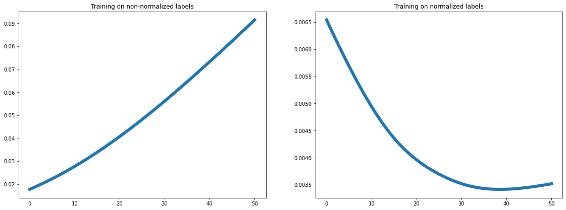
• Some features exhibit unexpected dependency plots. For instance, the model predicts less rainfall as there is more lightning (see the plot for atmosphere_instant_ltng) and it predicts low rainfall for low convective inhibition (surface_instant_cin). Upon further analysis, we found that data for the lighting and convective inhibition also follows this pattern, i.e., samples where there is less lightning have a higher average rainfall and where there is low convective inhibition there is low rainfall, respectively. But this is because the data for these features is sparse, and therefore the model is picking up on a spurious relationship. One way to correct the model for this feature was to train the model on normalized labels, and on doing so convective inhibition showed the expected dependency plot:

Feature Attributions

We use feature attributions to explain the behavior of the rainfall prediction model.

What is Feature Attribution?

A feature attribution technique attributes a machine learning model's prediction to its input features; influential features get higher attributions. Influence can either be positive (supporting the prediction) or negative (opposing the prediction). Typically, the prediction is a single scalar output, for instance for an object recognition task (e.g Imagenethttps://image-net.org/), the prediction is a probability of the image containing a specific object (e.g. a boat, or a tank, a specific dog breed etc.). The attributions identify which pixels are most influential to the prediction. In our case, there is a separate prediction for every one of the 256X256 locations. In a later section we discuss how to aggregate the attributions across locations; for now, let us imagine we have to explain predictions for a single location.

Saliency Maps

Feature attributions are visualized using images called saliency maps. Saliency maps have the same resolution as the input. For our rainfall prediction task, we display a separate saliency map (across a spatial grid) for every feature. On a saliency map, a pixel's shade determines its importance. In our visualizations, shades range from green for positive influence to purple for negative influence. The value of the saliency map at a specific pixel says how much that feature at that location contributed to rain in the selected output location(s).

Integrated Gradients

We use a feature attribution technique called Integrated Gradients. It has been used to explain a variety of deep-learning models across computer-vision, NLP, recommender systems, and other classification tasks.

Here is an informal description of Integrated Gradients. The technique operates by perturbing features. Intuitively, perturbing an important feature will change the score more substantially than perturbing an unimportant feature; an infinitesimal perturbation is a gradient of the score wrt the features. Integrated Gradients accumulates these gradients along a path that results from linearly varying each feature from a baseline value to actual input value. The baseline value for features selected so as to force the prediction of the model to near zero. (We discuss the selection of the baseline below). The score of the model therefore varies along this path from zero to the actual output value.

Mathematically, the attribution to a single feature \(i\) is defined as: $$ \phi (x_i) = (x_i - x_i') \int_{\alpha=0}^{1} \frac{\delta F(x_{\alpha})}{\delta x_i} d\alpha \cdots (1) $$ Here the input is \(x\), the baseline is \(x'\), \(F(x)\) is the output of model, \(\frac{\delta F(x_{\alpha})}{\delta x_i}\) is the gradient of \(F(x)\) along the \(i^{th}\) feature and \(x_{\alpha} = x' + \alpha \times (x - x')\).

Integrated Gradients satisfies several desirable properties, and in fact, uniquely so (see Corollary 4.4 here). We highlight one such property called 'completeness'. Integrated Gradients accounts for the change in the score from the baseline value to the actual output value. This is a simple consequence of the fundamental theorem of calculus; integrating derivatives (gradients for a multivariable function) between two points \(x\), \(x'\) yields the difference between the functions at the two points. That is, the sum of the attributions over all the input features is equal to \(F(x) - F(x')\). Since we select a baseline that sets \(F(x')\) to zero, the attributions can be interpreted as a redistribution of the score.

Baseline Selection

As discussed, we select a baseline so as to minimize the prediction of the model, i.e., set the predicted rainfall to zero. To do this, we leverage our one-at-a-time analysis. If the rainfall prediction is monotonically increasing in a feature, we set its baseline value to its trimmed minimum value (1st percentile). If the function is monotonically decreasing, we set the baseline value to the trimmed maximum value (99th percentile). The trimming is to ensure that our baselines aren't sensitive to outliers. If the function is convex or concave, we set the baseline at the single local minimum.

Using the described method we get a zero rainfall prediction.

Extending Integrated Gradients to Analyze Error

Feature attribution methods are typically used to study predictions. In this section, we extend the approach to apply to the model's error/loss. To the best of our knowledge, this is a novel application of feature attribution.

We will identify features that have a positive influence (decrease error) on the quality of the model's prediction on the input, versus those that have a negative influence (increases error). This analysis requires knowledge of the groundtruth, and can only be performed after it is available (once the three hours have elapsed in our case.)

We derive the analytical form of feature attributions for error. Let \(E\) denote the squared error of the model's prediction: $$ E(x) = (L(x) - F(x))^2$$ here \(L(x)\) is the label of the input.

We integrate the gradient of the error along the linear path (defined by the parameter \(\alpha\)) from the baseline \(x'\) to the input; here \(x_{\alpha}\) is a point along the path. Throughout this process, we hold the label fixed at its input value \(L(x)\); this quantity is the model's target. The attributions reflect how the model makes progress towards reducing (or increasing) error along this path.

The attribution for a feature \(i\) is: $$ \phi (x_i) = (x_i - x_i') \int_{\alpha=0}^{1} \frac{\delta (L(x) - F(x_{\alpha}))^2}{\delta x_i} d\alpha \cdots (2) $$ $$ \phi (x_i) = (x_i - x_i') \int_{\alpha=0}^{1} 2(F(x_{\alpha}) - L(x)) \frac{\delta F(x_{\alpha})}{\delta x_i} d\alpha \cdots (3) $$

The second step is via application of the chain rule: the gradient of the function \(E\) with respect to a feature can be written as the gradient of the function \(E\) with respect to the score \(F\) , which is \(2(F(x) - L)\) times the gradient of the score wrt the feature \(\frac{\delta F(x_{\alpha})}{\delta x_i}\)

Compare this to the expression in Equation 1. The difference from prediction attributions is the scaling by the term \(F(x) - L\) which changes the scale and sign of the gradients being accumulated.

Aggregating Attributions

Thus far, we have discussed how to identify influential features (with localities) for a prediction at a single location in the grid. However, this is not directly usable because as analysts/meteorologists, we would prefer explanations for a groups of locations such as a locality where rain is predicted everywhere, or a locality where the model is inaccurate, or on the entire 256X256 output grid, to understand the aggregate influence of individual features. It would be painful to communicate these explanations pixel by pixel. Fortunately, the attributions are in prediction units (i.e., in quantity of precipitation), therefore we can sum attributions for a set of output pixels; the attribution for a feature, location combination now corresponds to how much it contributes to the total rainfall in the selected output pixels.

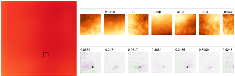
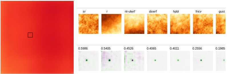
Using Rain Checker

You can inspect the prediction and error attributions and feature importance using the tool below in the following ways:

• Use the dropdown menu at the top to analyze prediction or error attributions.
• Select any of the first three images from the sample selector at the bottom to analyze individual samples.
• Select the last image in the sample selector to analyze the aggregate of attributions over 200 samples (global). We filtered out examples with high rainfall (> 3.5 mm) from this set, because we found that the model was severely underpredicting on these instances.
• The tool by default reorders the features by importance of increasing attributions or lowering loss. If you would like to study the effect of a specific feature across locations or samples, uncheck the box.
• Click around over the image in the second row to select different segments to analyze. Each segment has 16X16 pixels.
• The 'Total segment attribution' score is a sum of prediction / error of all pixels in the selected segment.
• The scores over attribution maps for each feature are a sum of the attributions over all the pixels for that input feature.
• Hover over the input feature or its corresponding attribution map to see a descriptive name for each feature.

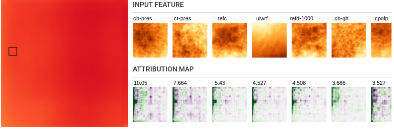
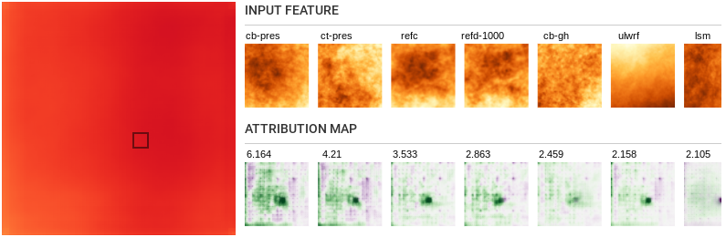
Learnings

1. Some features consistently receive high attribution across samples and locations, driving predictions and a reduction in error.
   • Maximum Radar Reflectivity (refc) and Radar Reflectivity at 1000m above ground level (refd-1000) consistently ranks in the top 5 features. This is expected because it is a direct measure of the rainfall (three hours before the prediction), and rainfall now is likely to imply rainfall later.
   • For low-medium rainfall regions \((>0.5mm/hr)\) cloud-top pressure (ct-pres) and cloud-base pressure (cb-pres) are consistently the top two input features. We know that tall, deep clouds are likely to produce precipitation, and these two features estimate the height and thickness of the cloud https://www.goes-r.gov/products/baseline-cloud-top-pressure.html.

   

   • When examining the global attributions, for most segments, upward longwave radiation flux (ulwrf) shows up as one of the top important features. It measures the amount of thermal radiation emitted by the Earth’s surface and clouds into the atmosphere. Low amounts of ULWRF are considered representative of deep convection and are used as a heuristic indicator of cloudiness and precipitation estimation .

   

2. Left to right influence:
   • We see that output pixels are regularly influenced by feature locations on the left of the pixel. This is likely due to the Coriolis effect https://en.wikipedia.org/wiki/Coriolis_force#Applied_to_the_Earth that creates winds blowing from west to east (Westerlies)https://en.wikipedia.org/wiki/Westerlies. One obvious consequence of this is that the model will likely not generalize to locations with different prevailing winds, say in south Asia. This also suggests that care should be taken in training models like this in regions with monsoonal circulation patterns.

   

3. Local influence:
   • For features like relative humidity (r) and total cloud cover (tcc), the location in the input corresponding to the selected output pixels has a positive influence on rain, however surrounding regions have a negative influence on rain.

   

   • Features such as frictional velocity (fricv), surface lifted index (lftx) and downward shortwave radiation flux seem to have a strong influence from the same region as the chosen segment and not much from other places around.

   

4. Border artifacts:
   • Notice that on analyzing segments close to the borders of the sample, especially the left border, we see high attribution values along the edges. This is however not the case for segments closer to the middle of the sample. This clearly shows that predictions at the border are weaker due to the lack of information from spaces outside the sample. This could help trim down our predictions to regions with high quality predictions.

   

Conclusion

We analyze a deep learning network that has superior accuracy in forecasting rainfall three hours out than HRRR, a forecast system based on traditional numerical weather prediction.

Our motivation was to check whether the deep learning model obeys causal patterns indicated by the physics of rainfall. We found this to be largely the case. The most influential features (pressure differentials, and measures of current rainfall) were as expected. However, we did notice breakages of causality as well. First, we found that the model predicted less rainfall with more lightning, an issue possibly stemming from the sparsity of data. Second, we found that rainfall predictions at a location tended to depend on sensor readings towards the left. This is a consequence of building a model on training data from the continental U.S., where the prevailing wind direction is left to right. This indicates that the same model wouldn't be suitable for predicting rainfall in other geographies. Perhaps adding features such as wind direction and ground elevation could produce a more causal model.

Finally, we expect our explainable, i.e., our feature attribution exploration widget, to apply to the influence of features on predictions and more importantly on the error/loss of the model, across a number of weather tasks including wind, solar energy, flood and wildfire prediction, that all share the characteristic of producing predictions across a spatial grid.